
Generating true randomness on a tiny microcontroller can be a real challenge. Many small MCUs, for all their versatility, lack built-in hardware sources of entropy, yet countless projects depend on high-quality randomness for security, simulation, and creative experimentation. In this post, we’ll look at how to extract genuine unpredictability from a simple, reliable circuit, using just four components to build a surprisingly effective hardware entropy source.
The Problem
When using the Arduino random() function, or any pseudorandom number generator, it’s up to the user to provide an initial seed. This seed should ideally be genuinely unpredictable. On a desktop PC, that’s easy: you can use the current date and time or pull high-quality entropy from a hardware source like /dev/random on Linux.
Neither option exists on a small microcontroller. The Arduino manual for random() suggests reading from a floating analog pin and using that value as a seed:
long randNumber;

void setup() {
  Serial.begin(9600);
  randomSeed(analogRead(0));
}

void loop() {
  randNumber = random(300);
  Serial.println(randNumber);
  delay(50);
}
There’s a number of issues with this approach:
The amount of entropy is unpredictable
A floating pin’s behaviour depends heavily on its environment. It might sit in a noisy, interference-rich setting—or in an electrically quiet one. Your project could be sealed inside a plastic enclosure or housed in a shielded metal box. It might run from noisy mains power or from a clean battery supply in the middle of no-where.
A better solution would be one that isn’t influenced by environmental factors and can deliver a predictable, consistent amount of entropy every time you need it.
A floating pin is coupled to predictable noise sources
Most sources of electrical noise are slow and largely predictable. When I plotted the output of analogRead(0) in my lab, the graph was dominated by the 50 Hz hum of the mains, an entirely predictable sine wave. This means that most of the bits produced by analogRead() are of very low quality.
Even worse, a floating pin is often capacitively coupled to the MCU and nearby circuits. Small changes in layout or operation can completely change any available “entropy,” sometimes even saturating the seed to all ones or all zeros. A small change to your layout may leave your project unintentionally malfunctioning or insecure.
A truly good source of entropy should derive most of its unpredictability internally, from thermal noise, quantum effects, or other stochastic physical processes, rather than relying on external and unreliable environmental noise.
A Solution
A common solution for generating hardware entropy is to use a reverse-biased diode junction to generate avalanche and tunneling noise. While this can be effective, it comes with several challenges: the output is highly sensitive to temperature and bias voltage, and the raw noise is difficult to harvest. This approach requires a carefully designed, complex analog front end to amplify and condition the signal before it can be interfaced with a microcontroller.
A diode-based white noise generator is ideal if you need to produce a large quantity of entropy. But if your goal is simply to generate enough high-quality entropy to seed a PRNG (possibly even a cryptographically strong one) then reliability and ease-of-use become the primary concerns.
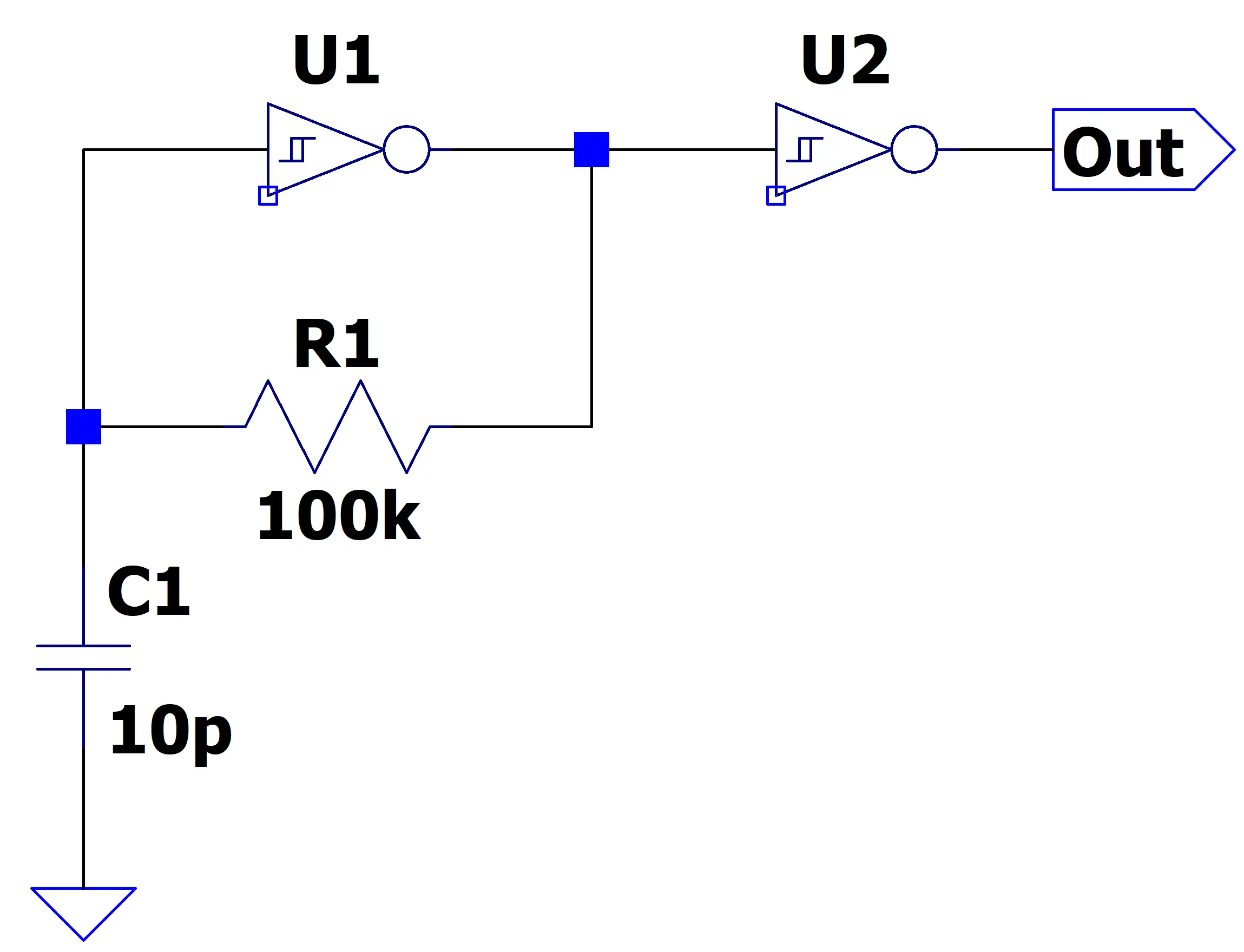
Well, I have something for you to try. A solution based a simple CMOS RC oscillator:
Parts you’ll need
- Assorted Resistors (AliExpress | Amazon)
- Assorted Ceramic Capacitors (AliExpress)
- TI SN74AC14N (LCSC)
- 1N4004 (AliExpress)
This oscillator is about as simple as it gets. When the output of U1 is high, C1 begins to charge through R1. As the capacitor voltage rises past U1’s upper trigger threshold, the inverter flips state and the output transitions from high to low. C1 now discharges through R1 until the voltage drops below the lower trigger threshold. The cycle then repeats, producing a continuous free-running oscillation.
A second inverter from the same package acts to buffer U1’s output. This buffer isolates the oscillator from external disturbances and ensures that any loading or noise from downstream circuitry doesn’t interfere with the core oscillation behavior.
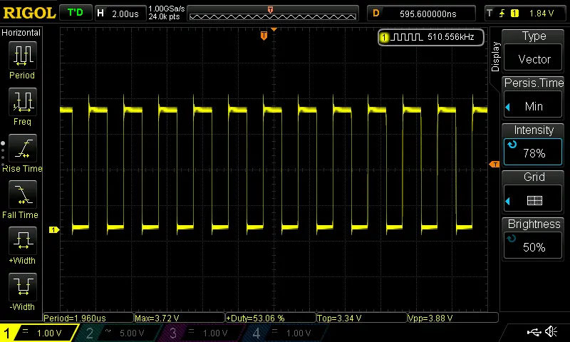
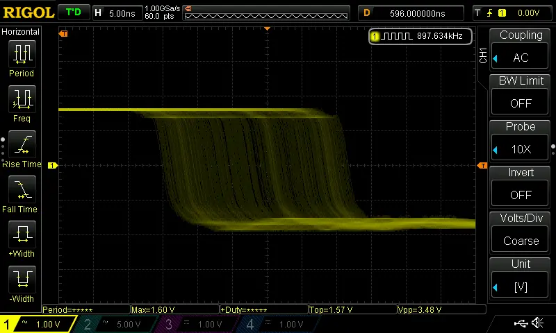
The output of this oscillator is a clean square wave, with close to a 50% duty cycle:
Uncertainty
At first glance, the square-wave output doesn’t seem useful for our purposes—it looks completely predictable. But when we zoom in on the first falling edge, something interesting appears. The transition isn’t perfectly sharp; instead, it forms a slight blur. Some edges occur a little earlier, others a little later. Jittering perhaps by about +-2ns.
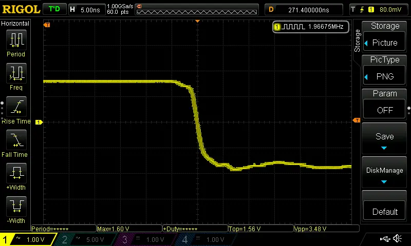
This tiny uncertainty is driven by thermal noise in R1 and by microscopic, quantum-scale variations in the movement of charge carriers inside the CMOS junctions of U1. These subtle effects cause C1 to charge a bit faster at times and a bit slower at others. And here’s the key: even though the jitter on any individual edge is very small, it accumulates over time.
Here is a diagram showing three separate samples of the same signal, all starting perfectly in phase. I’ve exaggerated the jitter for clarity:
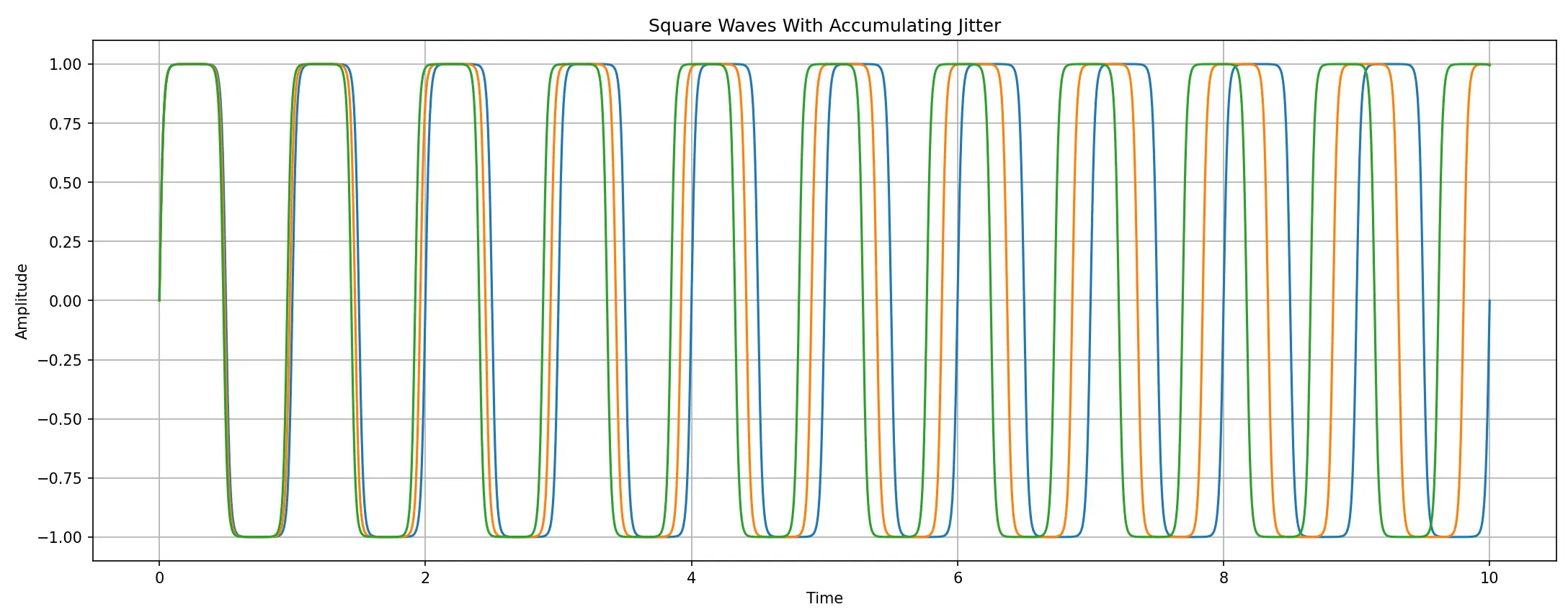
Within the first few wavelengths, the three signals are almost indistinguishable. But as time goes on, the accumulated jitter causes their phases to drift further and further apart. By the time we reach around ten wavelengths, the phase relationship has completely decorrelated — making it impossible to predict whether a digital sample taken at that moment will read as high or low.
There are a couple of great advantages to this approach:
- The signal is already at logic level, so we can sample it directly with digitalRead() — no analog front end, no level shifting, no fuss.
- The uncertainty comes from a truly unpredictable physical source, driven primarily by the thermal noise in R1
Even More Jitter
Although the base circuit already works, I wanted to see whether we could inject more noise into C1’s charging path. More jitter on each edge means fewer cycles until the phase relationship is unpredictable — which translates directly into more output bits per second.
Earlier I mentioned that diode-junction RNGs harvest white noise from avalanche or tunneling. Could we combine that raw noise with the oscillator approach to get the best of both worlds — the simplicity and logic-level output of a free-running oscillator plus the rich stochasticity of a diode?
After some experimenting, I’ve discovered the answer is yes: a small, modification to the Schmitt oscillator increases edge jitter without demanding a complex analog front end.
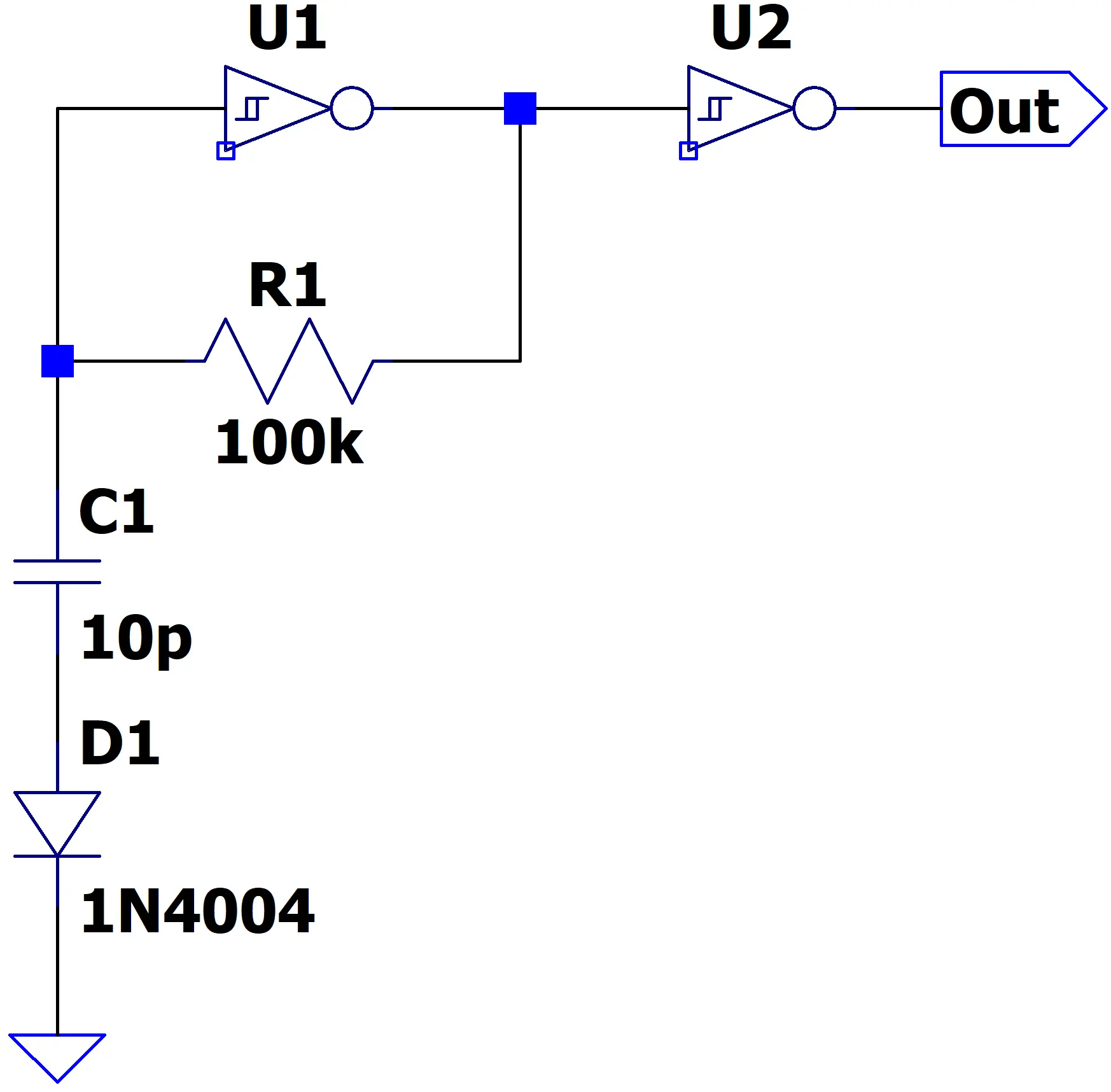
In the modified circuit above, I’ve made only a single, small change, to the original oscillator: Adding the 1N4004 rectifier diode, D1, in series with charging capacitor C1.
C1 blocks any DC component from reaching the diode. So D1 is exposed only to the AC portion of the signal at the inverter’s input. The trigger points of this inverter are only 1V apart, meaning the AC component of the signal is 1V peak to peak, or +-500mV.
This +-500mV is below the diode’s forward voltage of 700mV, so D1 doesn’t behave just as a diode in the usual sense—it behaves primarily as a small series capacitor.
A 1N4004 diode has a junction capacitance of approximately 10–15 pF. Because capacitors in series reduce the total capacitance, placing D1 in series with the original timing capacitor C1 effectively cuts the net capacitance of the RC network by about half. You can see the effect directly in the oscilloscope capture: the oscillator’s frequency nearly doubles once the diode is added.
C1 and D1 also form an AC voltage divider, splitting the ±500 mV swing between them according to their relative capacitances. When I probed the voltage across D1, I measured roughly ±220 mV, which is consistent with the two capacitors having nearly equal capacitance values.
So, what’s interesting about all of this? Well, let’s take a another look at the jitter on the falling edge of the signal now the diode is in place:
The amount of jitter observable on the first falling edge has increased dramatically, where we had about +-2ns of jitter before, now we have a whopping +-15ns, a total deviation of 30ns. At least a fifteen times improvement for the cost of a 10 cent diode.
Why does the diode increase jitter so dramatically?
The key is that the diode isn’t just acting as a small capacitor. At around 200 mV of forward bias, the diode becomes slightly leaky. A diode’s forward voltage isn’t a hard cutoff — it follows a smooth exponential curve — so even well below 700 mV it conducts a tiny current. When I measured the diode at roughly 200 mV, I saw about 100 nA of leakage. That doesn’t sound like much, but with the very small capacitances in this circuit, it’s enough to noticeably affect the final time constant.
That leakage current isn’t steady, either. It fluctuates due to a mix of thermal noise, carrier-generation noise, and shot noise inside the junction. Those microscopic variations directly modulate the charging current, which in turn injects jitter into the exact moment the Schmitt trigger threshold is crossed.
How Often To Sample The Oscillator?
If we sample too soon, there hasn’t been enough time for jitter to accumulate, and the resulting bits won’t be very random. But if we wait too long, we’re simply wasting time — generating entropy more slowly than the circuit is capable of.
Helpfully, I found a paper that addresses this very subject. We don’t need to go through the paper in detail, as it contains a simple formula that for a conservative estimates of the worst case entropy if we know the amount of accumulated jitter. The formula is:
Accumulated Standard Deviation (σₐ)
σₐ represents the standard deviation of the oscillator’s timing uncertainty at the moment we take a sample, expressed in wavelengths. For example, if the oscillator’s period is 100 ns and the measured jitter on each edge is ±5 ns, then the total variation is 10 ns — one tenth of the wavelength — giving:
σ = 0.10
As the oscillator runs, this timing uncertainty accumulates from cycle to cycle. Since each cycle’s jitter is uncorrelated, the accumulation behaves like a random walk, meaning the standard deviation after N cycles grows with the square root of N:
Probability of guessing the outcome (pₑ)
The value pₑ represents the probability that an attacker can correctly guess the result of sampling the oscillator, given an accumulated timing uncertainty (standard deviation) of σ. Our goal is to push pₑ as close to 0.5 as possible — meaning the best an attacker can do is no better than a coin flip.
Importantly, pₑ is a worst-case estimate, because it assumes the attacker:
- Knows the previous sample value,
- knows the exact phase of the oscillator at the moment that sample was taken, and
- knows the exact time that has elapsed since then, with perfect precision.
In a real system, these assumptions almost never hold. Any deviation — clock drift, scheduling jitter, external interrupts, or simply not knowing the exact sampling instant — all reduce the attacker’s predictive power. In practice, this means the actual probability of an attacker correctly guessing the next bit is worse (closer to 0.5) than the value predicted by the formula.
Entropy vs Deviation
To make things easier, I’ve taken the formulas from the paper and compiled them into the table below. Each row shows how the accumulated standard deviation (σₐ), measured in wavelengths, affects:
- pₑ — the attacker’s best-case probability of correctly guessing the sampled bit
- Entropy per bit — the amount of usable entropy in each output bit (1.0 is perfect)
As σₐ grows, the phase uncertainty increases, pₑ approaches 0.5, and the entropy per bit approaches the ideal value of 1.
| σₐ | pₑ | Entropy per bit (Ideally 1) |
| 0.1 | 0.848 | 0.238 |
| 0.2 | 0.722 | 0.471 |
| 0.3 | 0.632 | 0.662 |
| 0.4 | 0.575 | 0.799 |
| 0.5 | 0.541 | 0.885 |
| 0.6 | 0.523 | 0.936 |
| 0.7 | 0.512 | 0.965 |
| 0.8 | 0.507 | 0.981 |
| 0.9 | 0.503 | 0.990 |
| 1.0 | 0.502 | 0.995 |
Choosing a Sampling Interval
From this table, it becomes clear that we don’t need the accumulated jitter (σₐ) to reach a full wavelength to achieve high-quality entropy. Even at σₐ ≈ 0.5, each sampled bit already carries almost 0.9 bits of entropy, and by σₐ ≈ 1.0 we’re essentially at cryptographic quality. This gives us a practical guideline for choosing the sampling interval: wait just long enough for σₐ to reach the desired range, but no longer.
A Worked Example
In my implementation, I’m aiming for cryptographic-grade entropy, which means I want roughly one full wavelength of accumulated jitter between samples (σₐ = 1.0). Here’s how the numbers work out:
The oscillator runs at 900 kHz, giving a wavelength of:
The measured per-edge jitter is about 30 ns, corresponding to a normalized standard deviation of:
Using the random-walk relation for accumulated jitter:
We set σₐ = 1.0:
Solving for N:
Finally, converting cycles to a real-time delay:
This gives the interval at which to sample the oscillator to achieve roughly one wavelength of accumulated jitter per read.
Sampling Implementation
I built the circuit and used the following Python script on an Orange Pi Zero to sample the GPIO every 1.5 ms and write the results to a file:
import wiringpi as wp
import time

PIN_PC10 = 16
wp.wiringPiSetup()
wp.pinMode(PIN_PC10, wp.INPUT)

def read_rnd_byte():
    value = 0
    for i in range(8):
        bit = wp.digitalRead(PIN_PC10) & 1
        value = (value << 1) | bit
        time.sleep(0.0015)  # 1.5 ms
    return value


def stream_bytes_to_file(path):
    total_bytes = 0

    with open(path, "ab") as f:
        while True:
            b = read_rnd_byte()
            f.write(bytes([b]))
            total_bytes += 1

            if total_bytes % 64 == 0:
                print(f"{total_bytes / 1024:.2f} KB")

stream_bytes_to_file("output.bin")
I left this python script to run until I had gathered approximately 10MB of raw random data. I then analyzed the results using ent:
matty@latitude:~/Documents$ ent -b output.bin
Entropy = 0.996663 bits per bit.

Optimum compression would reduce the size
of this 81120552 bit file by 0 percent.

Chi square distribution for 81120552 samples is 374991.07, and randomly
would exceed this value less than 0.01 percent of the times.

Arithmetic mean value of data bits is 0.5340 (0.5 = random).
Monte Carlo value for Pi is 2.923091033 (error 6.96 percent).
Serial correlation coefficient is -0.000068 (totally uncorrelated = 0.0).
This is effectively a perfect result.
The minor reported loss of entropy and the slight deviation in the arithmetic mean are due to the oscillator’s duty cycle being about 53%, rather than a perfect 50%. If required, this bias can be removed using a whitening algorithm.
Using the Output for a Cryptographic Key
Even without whitening, these results are strong enough for use directly as the seed for a PRNG or even a cryptographic key
To illustrate, consider generating a 256-bit AES key directly from this raw hardware RNG output. With an entropy of 0.997 bits per bit, the total entropy for a 256-bit key is roughly:
This is effectively the full 256-bit security, meaning that even with the tiny bias, an attacker’s ability to guess the key is negligibly affected. You can safely feed the raw output directly into a cryptographic PRNG or key generation routine, without needing any additional post-processing. This is a rare feature for a hardware RNG, most need substantial processing to be this usable.
This generator is likely sufficient for casual use, but a high-security implementation should include, at minimum, generator health checks. As a defense-in-depth measure, you could also apply a whitening and mixing algorithm — for example, XORing the RNG output with a cryptographically strong stream cipher. One practical option is ChaCha20, which is fast, secure, and could even be seeded from a stored key in EEPROM, so that in the event of a PRNG failure, the system maintains resilience against a variety of attacks.
Visualizing the Output
As a visual sanity check, and for fun, I converted part of the gathered data into a black and white image, which would allow any obvious patterns to be viewed directly:

Looks good!
Conclusion
With just a handful of components — a Schmitt-trigger inverter, a resistor, a capacitor, and a simple diode—you can build a reliable hardware entropy source for the Arduino or similar microcontrollers. The output is genuinely random, derived directly from stochastic physical processes in the oscillator and diode junction. This circuit is unusually unbiased compared to typical hardware RNGs, and the raw output is already high-quality enough to seed a PRNG directly. While post-processing, such as whitening, can be applied in cryptographic or other applications requiring absolute perfection, it is entirely optional here. Compact, easy to implement, and requiring no complex analog front end, this approach provides a practical and robust solution for projects that rely on truly unpredictable numbers.


Leave a comment