
Today we’re going to look at crystal radio coils, and how you can build a good one. Not necessarily the best one, but one that delivers high performance for the materials available to you.
The coil is the fundamental component of any crystal radio. In conjunction with a tuning capacitor, it forms a resonant circuit that accumulates energy over multiple cycles of the radio signal. This type of circuit, commonly called an LC or tank circuit, functions analogously to a tuning fork or a playground swing. Each cycle of the radio wave adds additional energy into the tank circuit and the voltage keeps climbing until the energy added each cycle equals the energy lost each cycle.
The tank circuit’s role is twofold:
- Sensitivity: Boosting the voltage until it’s high enough to be detected.
- Selectivity: Favoring the desired frequency while rejecting others.
If you only want to see the measurements, you can jump to the results.
What is Q?
The tank circuit’s performance in both these roles is impacted by a unitless measurement known simply as Q — short for quality factor.
Q is simply the ratio of the total energy stored, over the energy lost per cycle. If the tank had 200 units of energy stored, and in that cycle it loses 1, the Q is 200.
A higher Q means less loss, so the voltage builds up more strongly. But Q has a second effect that’s less obvious: it also determines how narrow a slice of the radio spectrum the circuit responds to — its bandwidth. A high Q circuit is selective, a low Q circuit is broad. The relationship is:
This ratio gives you the -3dB bandwidth frequency — the frequency where an adjacent signal is only half the power. In practice you want the adjacent station to be attenuated far more than that — because half the power would still be clearly audible, so erring toward a narrower bandwidth gives you cleaner reception.
MW stations are spaced 9kHz apart (10kHz in the Americas). The bandwidth should be around this figure and ideally somewhat less — wide enough to receive the station clearly, narrow enough to reject its neighbours.
| Q | BW @ 500kHz | BW @ 1MHz | BW @ 1.5MHz |
|---|---|---|---|
| 50 | 10 kHz | 20 kHz | 30 kHz |
| 100 | 5 kHz | 10 kHz | 15 kHz |
| 150 | 3.3 kHz | 6.7 kHz | 10 kHz |
| 200 | 2.5 kHz | 5 kHz | 7.5 kHz |
| 250 | 2 kHz | 4 kHz | 6 kHz |
| 300 | 1.7 kHz | 3.3 kHz | 5 kHz |
| 350 | 1.4 kHz | 2.9 kHz | 4.3 kHz |
Looking at this table, anything with a Q over 100 will be functional — it will receive stations, but adjacent channel bleed is likely, particularly at the top of the band. A Q of around 150 is close to ideal across the MW band.
That said, having a higher Q than needed isn’t a problem — the detector and antenna coupling will consume energy from the tank, lowering the effective Q.
You can think of Q as a spendable resource: excess Q gives you headroom to trade for output volume, whereas low Q is a limitation you can’t easily overcome.
What is Self Resonant Frequency?
Every coil has a small amount of capacitance between its turns — called distributed or self-capacitance. This capacitance, combined with the coil’s inductance, forms a parallel resonant circuit all on its own, even with nothing connected to it.
The frequency at which this happens is the self-resonant frequency, or SRF.
For a crystal radio coil, this matters because the SRF sets a hard upper limit on the frequencies the coil can tune. If the SRF is too close to the operating frequency, the coil’s effective inductance shifts unpredictably and losses climb steeply. A good rule of thumb is to keep the SRF at least 2–3× above the highest frequency you intend to tune.
The SRF also sets a practical lower bound on your tuning capacitance. Since the self-capacitance appears in parallel with the tuning capacitor, the total capacitance in the tank circuit is the sum of the two. Even with the tuning capacitor at its absolute minimum, you can never have less capacitance than the coil’s own self-capacitance.
What You’ll Need
Manganese Zinc (MnZn) Ferrite Rod (AliExpress | Amazon)
500g Enameled Copper Wire (AliExpress | Amazon)
Litz Wire 50/100M (AliExpress | Amazon)
50g Enameled Copper Wire (AliExpress | Amazon)
Shorter Litz Wire (For ferrite core coils):
Litz Wire (10M AliExpress | 15M Amazon)
Other
Consumables. Wick, flux, etc (AliExpress | Amazon)
Measurement Methodology
Each coil (L1) was wound as close as practical to 250 μH. This value was chosen because, in conjunction with a 40–400 pF vintage air-variable capacitor (C1), it allows tuning across the entire MW broadcast band. The capacitor is the same type commonly used in traditional crystal radios.
C1 is then tuned to 1MHz, roughly the middle of the band. This ensures every coil is tested under conditions representative of actual use.
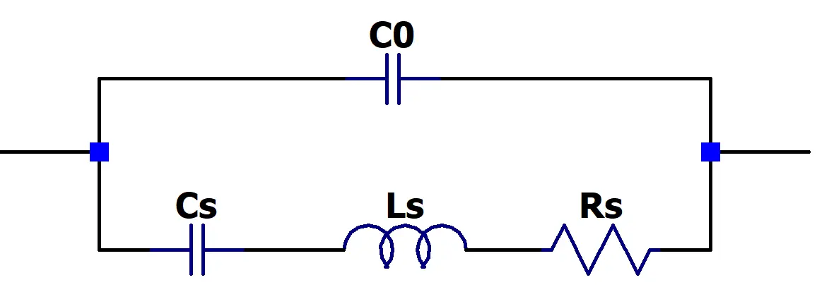
Schematic

Q
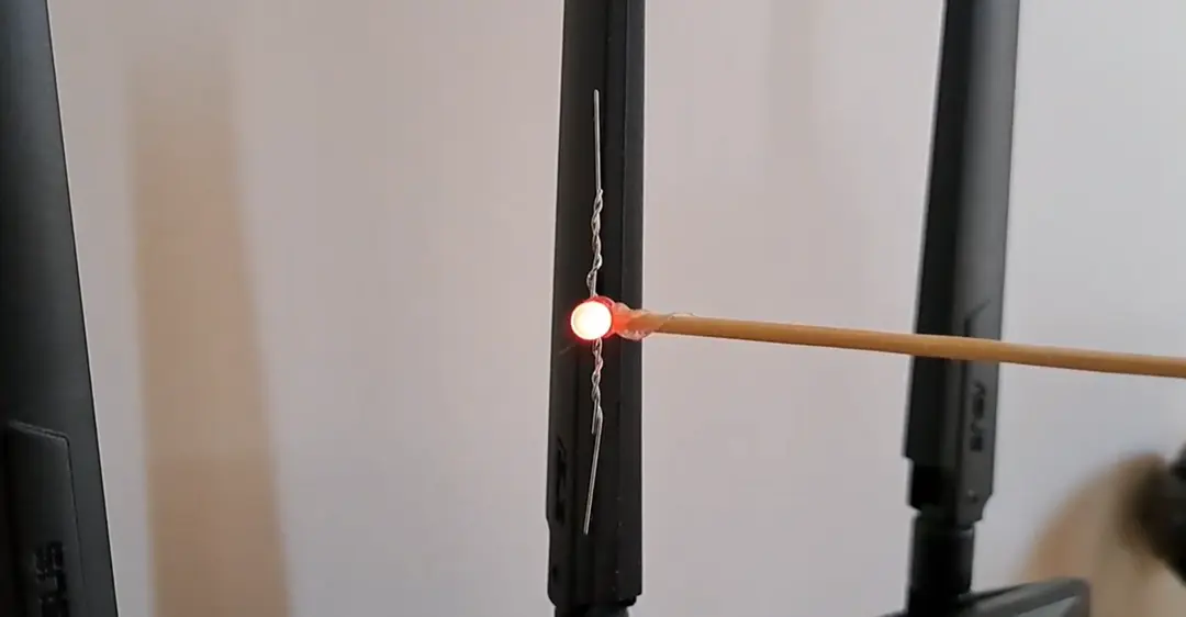
To measure Q, I used a ring-down method. The coil is briefly excited by a 10μs pulse injected through diode D1. The pulse runs from -2V to +2V, so between pulses the anode of D1 sits at -2V — firmly reverse biased and presenting no load to the tank during ring-down.
The pulse repetition rate is 1kHz, giving 1ms between pulses — ample time for the oscillation to decay fully before the next excitation.
The resulting ring-down is buffered by a RF JFET source follower and captured from OUT on an oscilloscope then processed in software.
C1 and C2 together present a series capacitance of 0.5pF, ensuring the LC circuit is very lightly loaded by the JFET buffer.
Q is extracted from the decay envelope using a Hilbert transform method, which is more robust to noise than identifying individual peaks. The envelope of the ring-down is fitted to a decaying exponential, and Q is calculated from the decay rate and resonant frequency using:
where α is the fitted decay rate in radians per second.
These measurements are intended as relative comparisons between coils rather than absolute Q values. However the test fixture is self-validating in a useful way — if the measurement circuit were introducing significant losses, the higher-Q coils would begin to bunch together near a ceiling set by the fixture rather than the coil itself. In practice the results are well spread, giving confidence that the fixture is not the limiting factor across the range tested.
SRF
To measure the self-resonant frequency, I used the same ring-down circuit described above, but with the variable capacitor C1 removed. With no external capacitance in the tank, the only capacitance present is the coil’s own distributed capacitance — so the frequency at which the circuit rings is, by definition, the SRF.
The measurement procedure was identical: a 10 μs pulse injected through D1 excites the coil, and the resulting ring-down is captured at OUT. The resonant frequency is extracted directly from the captured waveform.
Results
To compare coil designs on equal footing, I wound around a dozen coils across a range of wire types, core materials, and geometries, and measured each using a ring-down method. The results are ordered by Q below.
I only measured SRF for a select few coils, only enough to get an idea as to whether spiderweb winding was improving the coil’s SRF or not.
Q: 298
Inductance: 251 μH
Core: Spiderweb/Air
Wire: 0.05×50 litz
Turns: 61 ID 40mm OD 83mm
SRF: 4.42MHz


The standout performer of the entire test. With a Q of 298, this spiderweb coil handily takes the top spot, combining fine-strand litz wire with a geometry that minimizes proximity effect.
This is the coil to beat. It’s not the cheapest option, and winding a neat spiderweb takes patience, but if you’re chasing the highest possible Q, this is where the numbers point.
Interestingly, the SRF of 4.42 MHz is actually lower than several other coils tested, including the air-core litz solenoid at 4.90 MHz and the humble 0.3mm solenoid at 5.20 MHz. So despite the spiderweb’s reputation for low distributed capacitance, this particular winding doesn’t hold an advantage there — the higher turn count and larger overall diameter appear to offset any geometric benefit. The SRF is still comfortably above the MW band, but it’s worth noting that the Q win here is about loss reduction, not capacitance.
Q: 267
Inductance: 247 μH
Core: Solenoid/Air
Wire: 0.05×50 litz
Turns: 87 50mm OD
SRF: 4.90MHz


This air-core solenoid comes in 30 Q behind the litz spiderweb coil, but has the higher SRF of the two.
At approximately $6 of wire with no core required, it sits at a higher price point than the MnZn rod below but remains reasonably priced for a high performance coil.
The result confirms that litz wire addresses the proximity effect losses that limit solid wire solenoids, and that removing the ferrite core eliminates the core losses that limit the MnZn rod result. With both loss mechanisms addressed, this coil approaches what appears to be a practical ceiling for this geometry and frequency.
Q: 192
Inductance: 197 μH
Core: 100 mm MnZn Ferrite Rod
Wire: 0.07×15 Litz
Turns: 50
SRF: 4.10 MHz


With a Q of 192, this is one of the best performing coils tested — and also one of the cheapest. These 100mm MnZn ferrite rods are common and with the high permeability offered by the core, only 2M of litz wire is required.
It’s also much easier and faster to wind than many of the others.
Q: 173
Inductance: 252 μH
Core: 200 mm NiZn Ferrite Rod
Wire: 0.07×15 Litz
Turns: 48


Coming in close behind the MnZn rod, the NiZn rod also performs admirably. It should have a loss advantage at higher frequencies, but in the AM band it seems to be on equal footing with the MnZn rod. As these NiZn rods are less common and more expensive, there doesn’t seem to be much reason to choose one unless you are aiming for shortwave frequencies.
Q: 167
Inductance: 255 μH
Core: Spiderweb/Air
Wire: 0.8 mm
Turns: 54 40 mm ID 135mm OD
SRF: 4.2 MHz


This spiderweb coil demonstrates that thicker wire can yield higher Q, though the close-wound 0.8mm solenoid achieves virtually the same result — suggesting that for 0.8mm wire, spiderweb geometry offers no meaningful advantage. This coil provides reasonable performance but requires 15M of 0.8mm copper wire, making it significantly more expensive than the 0.3mm solenoid for a modest Q improvement.
Q: 164
Inductance: 254 μH
Core: Solenoid/Air
Wire: 0.8 mm
Turns: 80 60mm OD
SRF: 4.40MHz


The 0.8mm solenoid achieves virtually the same Q as the 0.8mm spiderweb coil, despite being close-wound. This suggests that for this wire diameter, spiderweb geometry offers no meaningful benefit — the proximity effect losses in the solenoid and the geometric penalty of the spiderweb appear to roughly cancel out. At around 9x the copper cost of the 0.3mm solenoid for a modest Q improvement, it’s hard to justify unless you already have the wire.
Q: 152
Inductance: 252 μH
Core: Solenoid/Air
Wire: 0.3 mm
Turns: 70 50mm OD
SRF: 5.20MHz


The 0.3mm solenoid sits in the middle of the pack and is the pragmatic choice for most builders — easy to wind, cheap to build, and performance that comfortably clears the selectivity threshold. It uses 1/9th as much copper by weight as the 0.8mm designs and costs around 1/9th the price, for only a modest reduction in Q.
It’s also worth noting that this coil achieved the highest SRF of any tested, giving it the most comfortable capacitance headroom at higher frequencies.
Coil32 provides accurate calculations for these coils, including estimated Q, distributed capacitance, and self-resonant frequency. While Coil32 predicts 0.3mm as the optimal wire diameter, measurements show 0.8mm wire achieves somewhat higher Q — however the cost difference makes 0.3mm the clear value choice for most builders. Deviating significantly from the 50mm former causes a steep reduction in Q, so stick close to that diameter if you can.
Q: 138
Inductance: 234 μH
Core: Spiderweb/Air
Wire: 0.3 mm
Turns: 58 40 mm ID 76 mm OD
SRF: 4.56MHz


The spiderweb coil was an interesting result — conventional wisdom dictates that spiderweb coils unconditionally grant higher Q due to lower capacitance. These results prove otherwise, with the 0.3mm spiderweb coming in slightly behind the 0.3mm air-core solenoid.
Both coils had a self-capacitance of under 2pF and an SRF over 4MHz, so neither had a capacitance issue in the MW band. The primary benefit of spaced winding in the MW band is a reduction in proximity effect losses — and it seems you need thicker wire to take advantage of it.
Q: 135
Inductance: 246 μH
Core: 200mm NiZn Ferrite Rod
Wire: 0.3 mm
Turns: 45


The NiZn ferrite rod is somewhat lacklustre when wound with 0.3mm enamel wire. There doesn’t seem to be much reason to choose this configuration when the 0.3mm air-core solenoid offers significantly higher performance for less cost and similar effort.
The ferrite cores seem to only shine when paired with a few meters of litz wire.
Q: 99
Inductance: 248 μH
Core: 200 mm NiZn Ferrite Rod
Wire: 0.8 mm
Turns: 50


Using close-spaced 0.8mm wire on the ferrite rod significantly reduces performance. The reason for this isn’t entirely clear, but the effect is pronounced and repeatable. My speculation is that the thicker wire’s larger surface area increases capacitive coupling to the ferrite.
It would be interesting to see if spacing the wire restores some of the lost performance.
Q: 60
Inductance: 220 μH
Core: 100 mm MnZn Ferrite Rod
Wire: 0.8 mm
Turns: 59


This result dramatically illustrates the importance of wire selection on ferrite cores.
Despite using the same MnZn rod that achieved Q of 178 with litz wire, switching to 0.8mm solid wire drops the Q to just 60 — less than a third.
The ferrite core appears to heavily penalize a longer coil length, making wire selection even more critical than with air-core designs.
Q: 31
Inductance: 247 μH
Core: Jaycar Toroid
Wire: 0.8 mm
Turns: 15


Worst performer. This ferrite core seems no good for high Q operation in the MW band.
This toroid was material L15 and came from jaycar. It may be intended primarily for chokes.
There are toroidal cores that should perform well — the Fair-Rite FT-140-61 has a good reputation in this role, but I don’t have any. Use my affiliate links or buy me a coffee if you want to encourage further testing.
Summary
Across all coils tested, a few clear patterns emerge. Ferrite cores only deliver their potential when paired with litz wire — solid wire on a ferrite core consistently underperforms the equivalent air-core winding.
Spiderweb coils likewise only yielded any significant benefit when wound with litz wire. However, the litz wire spiderweb delivered the highest Q out of all the coils tested.
Against conventional wisdom, I was unable to demonstrate that spiderweb distributed capacitance was lower than that of a solenoid. I cross-validated using several measurement approaches:
- Unloaded ring-down
- Resonance in parallel with a known test capacitance
- Frequency sweep with a VNA, checking phase for zero crossing
- Frequency sweep for peak amplitude when driven by a function generator
All methods agreed: the SRF of the spiderweb coils was lower than that of the solenoids. Perhaps the geometry wasn’t optimal, or the SRF advantage only appears at a different inductance than the 250 μH used here.
The spiderweb coils required more wire length to achieve the same inductance; the additional distributed capacitance from this may offset any benefit from the spaced winding. The greater physical area may also contribute more capacitance to the surrounding environment.
The MnZn rod with litz is the standout result: among the highest Q tested, good SRF, lowest wire cost, and easy to wind.
For builders on a budget, the 0.3mm air-core solenoid on a 50mm former is the pragmatic choice — cheap, simple, and performance that clears the Q and SRF thresholds comfortably.
Any new results will be added to this article as they become available.


Leave a Reply